Everything About Recursion in C++ [5]
This blog dives deep into recursion in C++, explaining its principles, practical examples like the Tower of Hanoi and Fibonacci sequence, and real-world applications to enhance your understanding of this fundamental concept.
Fri, Dec 20, 2024
11 min read

Table of Contents
Congratulations!
You've thoroughly explored this topic!
Table of Contents
Congratulations!
You've thoroughly explored this topic!
1. Introduction to Recursion
1. What is Recursion?
Recursion is a programming technique where a function calls itself to solve smaller instances of a problem until it reaches a base case. It is particularly useful for solving problems that can be broken down into simpler, self-similar problems.
2. Description
Recursion leverages the divide-and-conquer approach to solve complex problems by breaking them into manageable sub-problems. Each recursive call works on a smaller part of the original problem, eventually combining the results to produce the solution. Common use cases include tree traversals, combinatorial problems, and mathematical sequences like Fibonacci and factorial.
3. When is Recursion Useful?
Recursion is useful for problems that:
- Can be represented in terms of smaller instances of the same problem.
- Have a clear base case that terminates the recursion.
Examples include finding the factorial of a number, solving the Tower of Hanoi, and computing Fibonacci numbers.
4. Iterative Approach vs Recursive Approach
Let's compare iterative and recursive approaches using the factorial of a number as an example.
Factorial (Iterative Approach):
cpp1.int factorialIterative(int n) {2.int result = 1;3.for (int i = 1; i <= n; i++) {4.result *= i;5.}6.return result;7.}
Factorial (Recursive Approach):
cpp1.int factorialRecursive(int n) {2.if (n == 0) return 1; // Base case3.return n * factorialRecursive(n - 1); // Recursive case4.}
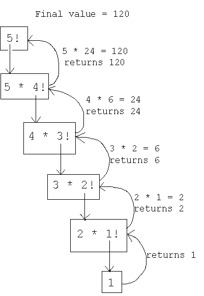
Suppose we want to find the factorial of 5. The iterative approach uses a loop to multiply numbers from 1 to 5, while the recursive approach breaks down the problem into smaller sub-problems until it reaches the base case as shown below:
5. Comparison:
| Aspect | Iterative Approach | Recursive Approach |
|---|---|---|
| Memory Usage | Efficient, uses a single stack frame | Less efficient, creates a new stack frame for each call |
| Complexity | Easier to debug and understand | May lead to stack overflow if not handled properly |
| Code Length | Longer and repetitive | Compact and elegant |
6. Cases in Recursion
-
Base Case
The condition where recursion stops. For example, in the factorial calculation, the base case isn == 0. -
Recursive Case
The part of the function where the problem is divided into smaller sub-problems. In factorial, this isn * factorial(n - 1).
7. Characteristics of Recursion
- Base Case: Every recursion must have at least one base case to avoid infinite loops.
- Progression: Each recursive call must move closer to the base case.
- Call Stack: Recursive calls use the program's call stack, which may lead to stack overflow if not managed correctly.
8. Difference Between Recursion and Iteration
| Feature | Recursion | Iteration |
|---|---|---|
| Definition | Function calls itself | Looping construct (for, while, etc.) |
| Termination | Base case is required | Controlled by loop conditions |
| Memory Usage | Uses stack memory | Uses heap/stack memory |
| Use Case | Best for problems with self-similar sub-problems | Best for problems with fixed or predefined iterations |
Example of Iteration:
cpp1.for (int i = 0; i < 10; i++) {2.// Iterative logic here3.}
Example of Recursion:
cpp1.void recursiveFunction(int n) {2.if (n == 0) return; // Base case3.recursiveFunction(n - 1); // Recursive call4.}
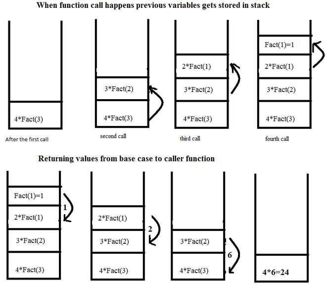
9. Visual Representation of Recursion Stack
2. Types of Recursion
Recursion can be broadly categorized based on the way the function calls itself and the position of the recursive call. Let's explore two key classifications:
1. Direct and Indirect Recursion
Direct Recursion
In direct recursion, a function directly calls itself.
Example: Calculating the factorial of a number.
cpp1.int factorial(int n) {2.if (n == 0) return 1; // Base case3.return n * factorial(n - 1); // Recursive case4.}
Indirect Recursion
In indirect recursion, a function calls another function, which in turn calls the first function. Example: Two functions alternately decrement a value until a base condition is met.
cpp1.void functionA(int n);2.void functionB(int n);3.4.void functionA(int n) {5.if (n <= 0) return; // Base case6.functionB(n - 1); // Calls another function7.}8.9.void functionB(int n) {10.if (n <= 0) return; // Base case11.functionA(n - 2); // Calls back the first function12.}
2. Tail and Non-Tail Recursion
Tail Recursion
In tail recursion, the recursive call is the last operation performed by the function. There are no pending operations after the recursive call, making it easier for the compiler to optimize using tail-call optimization. Example:
cpp1.int tailFactorial(int n, int accumulator = 1) {2.if (n == 0) return accumulator; // Base case3.return tailFactorial(n - 1, n * accumulator); // Recursive call at the end4.}
Advantages:
- Space-efficient due to tail-call optimization.
- Reduces the size of the recursion stack.
Non-Tail Recursion
In non-tail recursion, the recursive call is followed by additional operations. These pending operations prevent tail-call optimization. Example:
cpp1.int nonTailFactorial(int n) {2.if (n == 0) return 1; // Base case3.return n * nonTailFactorial(n - 1); // Recursive call not at the end4.}
Disadvantages:
- Requires more stack memory as operations are pending after the recursive call.
3. Key Differences Between Tail and Non-Tail Recursion
| Feature | Tail Recursion | Non-Tail Recursion |
|---|---|---|
| Position of Call | Recursive call is the last operation | Recursive call is followed by other operations |
| Optimization | Can be optimized by the compiler | Cannot be optimized due to pending operations |
| Memory Efficiency | More memory-efficient | Less memory-efficient |
3. Fibonacci Series Using Recursion
The Fibonacci sequence is a series of numbers where each number is the sum of the two preceding ones, starting with 0 and 1.
1. Description
- The Fibonacci series starts with
F(0) = 0andF(1) = 1. - Each subsequent number is computed as
F(n) = F(n-1) + F(n-2). - Using recursion, we can break the problem into smaller sub-problems until we reach the base cases (
F(0)andF(1)).
2. Steps to Compute Fibonacci Using Recursion
- Define the base cases:
- If
n == 0, return0. - If
n == 1, return1.
- If
- For other cases (
n > 1):- Recursively compute
F(n-1)andF(n-2). - Add their results to get
F(n).
- Recursively compute
- Combine the results to form the Fibonacci series.
3. Pseudocode
plaintext1.function fibonacci(n):2.if n == 0:3.return 04.if n == 1:5.return 16.return fibonacci(n-1) + fibonacci(n-2)
4. Implementation in C++
cpp1.#include <iostream>2.using namespace std;3.4.int fibonacci(int n) {5.if (n == 0) return 0; // Base case6.if (n == 1) return 1; // Base case7.return fibonacci(n - 1) + fibonacci(n - 2); // Recursive call8.}9.10.int main() {11.int n;12.cout << "Enter the number of terms: ";13.cin >> n;14.15.cout << "Fibonacci series: ";16.for (int i = 0; i < n; i++) {17.cout << fibonacci(i) << " ";18.}19.return 0;20.}
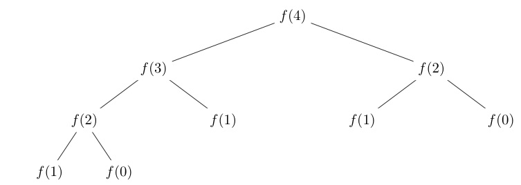
5. Recursion Tree for Fibonacci (F(4))
To compute F(4), the recursion tree would look like this:
text1.. F(4)2./ \3.F(3) F(2)4./ \ / \5.F(2) F(1) F(1) F(0)6./ \7.F(1) F(0)
4. Recursion Tree
A recursion tree is a visual representation of the recursive calls made by a function. It illustrates how a problem is broken down into smaller sub-problems and how the solutions are combined. Each node in the tree represents a function call, while its child nodes represent the sub-problems it spawns.
For example, in the Fibonacci sequence, the recursion tree for F(4) shows that F(4) is calculated as F(3) + F(2), and each of these calls further breaks down into smaller Fibonacci calculations until the base cases F(1) and F(0) are reached.
While recursion trees help in understanding the flow of recursive calls, they also highlight inefficiencies like repeated calculations (e.g., F(2) is computed multiple times in the Fibonacci example). This visualization emphasizes the importance of optimization techniques like memoization to improve performance.
5. Tower of Hanoi
1. What is the Tower of Hanoi?
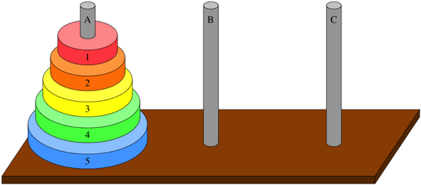
The Tower of Hanoi is a mathematical puzzle consisting of three rods and a number of disks of different sizes. The objective is to move all the disks from the source rod to the destination rod, following a set of rules, using the auxiliary rod as a helper.
It is a classic problem to understand recursion and its applications in solving problems with repetitive, self-similar steps.
2. Rules of the Game
- Only one disk can be moved at a time.
- A disk can only be placed on top of a larger disk or an empty rod.
- All disks start on the source rod and must be moved to the destination rod following the above rules.
3. Algorithm for Tower of Hanoi
To solve the Tower of Hanoi with n disks:
- Move the top
n-1disks from the source rod to the auxiliary rod. - Move the largest disk (nth disk) from the source rod to the destination rod.
- Move the
n-1disks from the auxiliary rod to the destination rod.
4. Pseudocode
plaintext1.function towerOfHanoi(n, source, destination, auxiliary):2.if n == 1:3.print "Move disk 1 from source to destination"4.return5.towerOfHanoi(n-1, source, auxiliary, destination)6.print "Move disk", n, "from source to destination"7.towerOfHanoi(n-1, auxiliary, destination, source)
5. Implementation in C++
cpp1.#include <iostream>2.using namespace std;3.4.void towerOfHanoi(int n, char source, char destination, char auxiliary) {5.if (n == 1) {6.cout << "Move disk 1 from " << source << " to " << destination << endl;7.return;8.}9.towerOfHanoi(n - 1, source, auxiliary, destination);10.cout << "Move disk " << n << " from " << source << " to " << destination << endl;11.towerOfHanoi(n - 1, auxiliary, destination, source);12.}13.14.int main() {15.int n;16.cout << "Enter the number of disks: ";17.cin >> n;18.19.cout << "The sequence of moves is: " << endl;20.towerOfHanoi(n, 'A', 'C', 'B'); // A: source, C: destination, B: auxiliary21.return 0;22.}
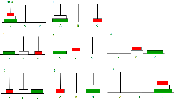
6. Recursion Tree for Tower of Hanoi (3 Disks)
For 3 disks, the recursion tree looks like this:
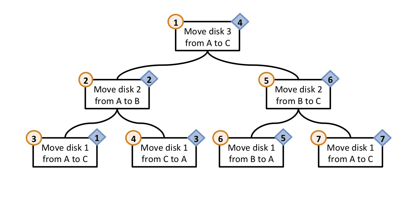
Each node represents a call to solve the problem for a specific number of disks. The branches show the recursive breakdown of sub-problems.
7. Example Execution for 3 Disks
- Move disk 1 from
AtoC. - Move disk 2 from
AtoB. - Move disk 1 from
CtoB. - Move disk 3 from
AtoC. - Move disk 1 from
BtoA. - Move disk 2 from
BtoC. - Move disk 1 from
AtoC.
8. Key Observations
- Number of Moves: The minimum number of moves required is
2^n - 1, wherenis the number of disks. - Space Complexity: O(n) due to the recursive stack.
- Time Complexity: O(2^n) since the number of moves grows exponentially with the number of disks.
6. Applications of Recursion
Recursion is widely used in solving various computer science problems, including:
- Sorting Algorithms: Algorithms like MergeSort and QuickSort use recursion to divide and conquer sub-arrays.
- Searching Algorithms: Binary search uses recursion to search through sorted arrays by repeatedly halving the search space.
- Tree Traversals: Recursion is used in tree structures for operations like Inorder, Preorder, and Postorder traversal.
- Dynamic Programming: Problems like Fibonacci and Knapsack are solved recursively, often optimized with memoization.
- Combinatorics: Generating permutations and combinations uses recursion to explore all possible combinations.
- Backtracking: Recursion is used in solving problems like n-Queens or Sudoku, where paths are explored and backtracked.
7. Conclusion
Recursion is a powerful technique that simplifies solving problems with a repetitive, self-similar structure. It is commonly used in algorithms, tree operations, and combinatorics. While it is elegant and intuitive, recursive solutions can be inefficient due to excessive function calls. Optimizations like memoization and tail recursion help improve performance. Mastering recursion is essential for solving complex problems and optimizing algorithms effectively.
Happy Coding! ✨